Physical Address
304 North Cardinal St.
Dorchester Center, MA 02124
Physical Address
304 North Cardinal St.
Dorchester Center, MA 02124

All about Graph pathfinding algorithms. How they work, the data structures they use, their time and space complexity, and practical use cases. Use this article as a learning resource and a technical reference guide.

Graph traversal systematically visits vertices. Depth‑First Search dives deeply along paths; Breadth‑First Search expands layer by layer. Built‑ons like topological sort and component detection exploit these passes to order DAGs and expose connectivity.

Discover how sorting algorithms, from bubble to quick, merge, heap, shell, and non‑comparison methods like counting, radix, and bucket, organize data efficiently, highlighting speed, memory use, and stability.

Dive into graph traversal: BFS for shortest unweighted paths, DFS for exhaustive discovery, plus weighted variants—Dijkstra, A*, bidirectional, and heuristic search. Understand frontier control and edge‑cost strategy for optimal exploration.

This article will guide and help you explore search methods and algorithms tailored to core data structures: linear & binary scans in arrays, O(1) hash lookups, prefix tries, balanced BSTs, skip lists, and B‑trees, mechanics, trade‑offs, and practical use cases.

This comprehensive guide demystifies search algorithms, from simple linear scans to hash‑table lookups, tries, balanced trees, and BFS/DFS in graphs. All while showing you how each strategy slashes lookup time for specific data shapes and teaching you how to write efficient code.

This article is a comparison chart and also a technical reference sheet which integrates provenance, algorithmic variants and engineering pragmatic factors (speed, memory, scope, etc.) of several popular Sorting Algorithms. Use this article as an advanced technical reference.

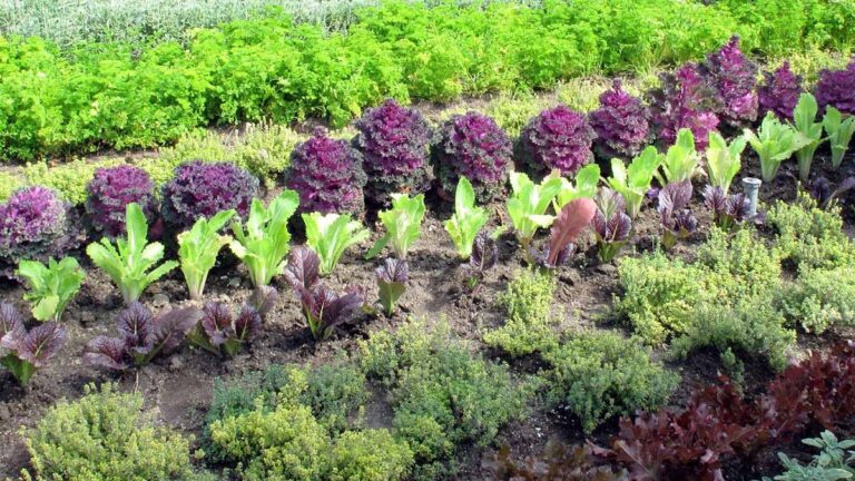
You don't need a big plot of land to grow carrots, radishes, leafy greens and other vegetables, as a matter of fact you don't need any land!, you can grow a surprisingly large amount of these edible plants and onions just using jars, pots, half-barrels and other small containers. This tutorial will guide you through the process in a friendly and easy to follow manner.
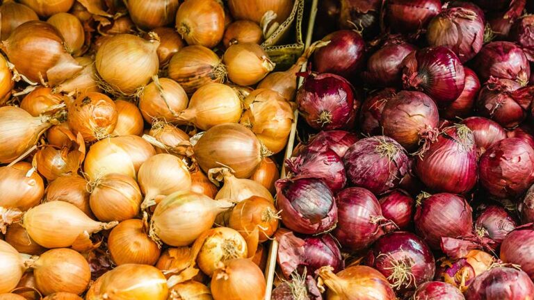
You don't need a big plot of land to grow garlic and onions, as a matter of fact you don't need any land!, you can grow a surprisingly large amount of garlic and onions just using jars, pots, half-barrels and other small containers. This tutorial will guide you through the process in a friendly and easy to follow manner.
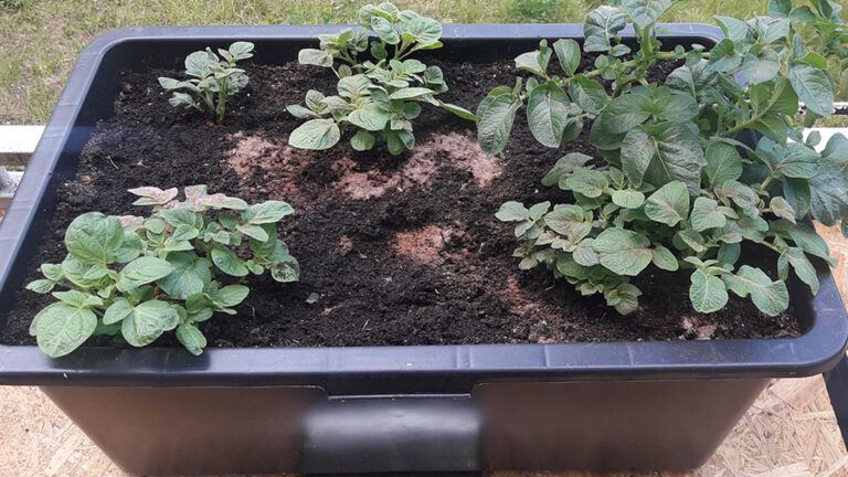
You don't need a big plot of land to grow potatoes, as a matter of fact you don't need any land!, you can grow a surprisingly large amount of potatoes just using jars, pots, half-barrels and other small containers. This tutorial will guide you through the process in a friendly and easy to follow manner.
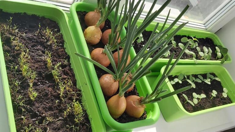
This tutorial will guide you through the fun and rewarding process of growing food in small containers. From potatoes, garlic and onions, to carrots and even leafy greens. Learn the grow cycles, the soil requirements and the different setups for indoor and outdoor planting.
Data layering in GIS is a fundamental technique that enables the creation of rich, informative maps by combining multiple data sources. Whether you are overlaying drone imagery with cadastral parcel lines or combining geological maps with weather data, this article will offer you a comprehensive guide.

Whether you are a new programmer or brushing up on fundamentals, this guide will help you understand these essential algorithms in a clear, tutorial-friendly way. From sorting, searching, graphing and cryptography to dynamic programming, greediness and machine learning algorithms.
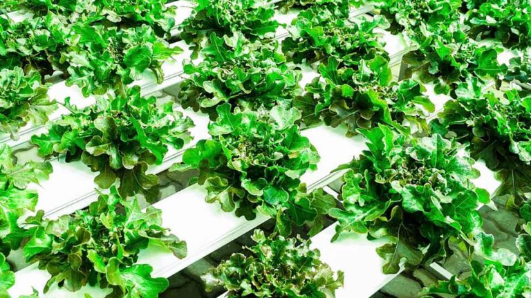
NFT hydroponics is an accessible and rewarding method for home gardeners to grow fresh produce and herbs. This guide and tutorial will teach you how to create your first NFT hydroponics setup at home, and then upgrade it in scale: Materials needed, assembly steps, crop types, and much more.

The ultimate, easy to read and understand guide and reference sheet to Vitamins. From the Role in the boy and the Recommended daily intakes, to the Food sources providing them and warnings about toxicity and other risks.

The ultimate, easy to read and understand guide and reference sheet to Essential Minerals & Electrolytes. From the Role in the boy and the Recommended daily intakes, to the Food sources providing them and warnings about toxicity and other risks.
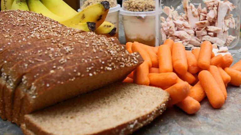
The ultimate, easy to read and understand guide and reference sheet to Key Nutrients, Antioxidants & Phytochemicals. From the Role in the boy and the Recommended daily intakes, to the Food sources providing them and warnings about toxicity and other risks.
The objective of this guide is to help and guide you to successfully create your own fully edible, near-closed-loop Edible Indoors Garden using techniques that range from hydroponics and vertical stacks, to microgreens and algae thanks: plant potatoes, seeds, legumes, leafy green, mushrooms and much more fully indoors.
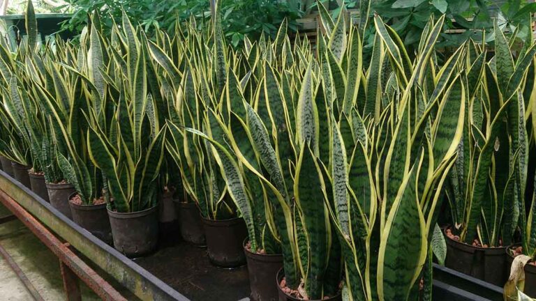
This guide will help you chose indoor plants based on a list of plant care factors that determine how easy or hard to maintain each plant is. Do you want an indoor plant that requires little care? Or do you want an exotic, beautiful indoor plant? This list will help you choose one.

By integrating digital design with data management tools, Building Information Modeling (BIM) techniques and technologies are revolutionizing architecture, engineering and construction (AEC) design. This comprehensive guide will help you understand and implement BIM.