Data Layering in GIS: Combining Multiple Data Layers in Maps

Introduction

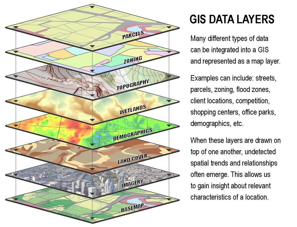
Geographic Information Systems (GIS) rely on the concept of data layering to organize and combine various types of geographic information into a single map or analysis. A layer in GIS is essentially one set of related data – for example, a road network, elevation measurements, or land use zones – covering the same geographic area. By stacking such layers together, a GIS map becomes a composite view of different information sources all aligned in one coordinate space. This approach lets users see how different aspects of the landscape relate to each other and forms the foundation for most GIS analysis and visualization.

Each GIS layer can be thought of as a transparent map overlay containing one theme of data. Keeping data separated by theme makes it easier to manage and visualize. For instance, one layer might contain only rivers, another layer only roads, and another population data. Separating information this way means each layer can be edited, styled, or analyzed independently, then combined as needed to create a full picture. It also reflects how data is often collected – a surveying team might collect roads and utilities as one dataset, while another source provides an imagery layer – which naturally lends itself to layering.

Note: this article is about the methods, approaches and techniques regarding the combination and merging of Information Layers in maps. For an introductory and detailed article about Geographic Information Systems (GIS) see: An Introduction to Geographic Information Systems (GIS) and Current GIS Technologies.

Key Concepts

Data Types – Vector vs. Raster

GIS data generally comes in two main forms. Vector data represents geographic features with precise geometry: points, lines, and polygons (for example, a point for a well location, a line for a road, or a polygon for a lake). Vectors are ideal for discrete features and have the advantage that they don’t lose detail when zoomed in. Raster data, on the other hand, is pixel-based and represents continuous surfaces or imagery. Aerial photographs, satellite images, and elevation grids are rasters (comprised of many cells, each with a value like color or height). Rasters are great for capturing details of continuous phenomena and visuals, but they have a fixed resolution (zooming in too far will show pixelation). GIS software allows layering of both types together – for example, placing vector roads on top of a satellite image raster – so understanding both is important.

Projections and Coordinate Systems

Because the Earth is round but maps are flat, every GIS layer is defined in a coordinate system (also called a projection when it’s a flat map) that specifies how coordinates in the dataset map to real locations on Earth. There are many coordinate systems in use; for example, one layer might use latitude/longitude coordinates (a global geographic system), while another uses a projected grid like UTM (Universal Transverse Mercator) or a local state plane system. Layers will not line up correctly unless they are using the same coordinate reference. A core task in GIS layering is ensuring all data shares a common projection or is appropriately transformed so that the layers align. Modern GIS tools can project data on the fly if the coordinate system for each layer is known, but it’s good practice to confirm and, if necessary, convert layers to a common coordinate system before analysis. In short, coordinate consistency is critical: a road layer in one projection and a satellite image in another must be brought into alignment, or the roads might appear offset from their true positions on the image.

Metadata

Simply put, metadata is “information about the data itself”. Along with the data itself, each GIS layer usually comes with metadata – information about the data. Metadata describes properties such as the coordinate system and projection used, the date the data was captured, its resolution or scale, the source or creator, and the accuracy or quality of the data. This “data about the data” is essential for effective layering. For example, without metadata you might not realize an aerial image uses a different datum (reference ellipsoid for coordinates) than your other layers, leading to misalignment. Or you might not know that a geological map layer was surveyed in 1970, making it potentially outdated compared to a recent drone image. Keeping track of metadata helps you properly align layers, respect the scale (using a dataset only at appropriate zoom levels), and understand any limitations. In practice, always check the metadata of each layer so you know how to handle it in your GIS project.

The Data Layers

GIS maps can incorporate layers from a wide variety of sources. Common data sources include:

Surveying data: Detailed measurements collected on the ground by surveyors or GPS units. These could be points (e.g. control points, utility markers), lines (property boundaries, road centerlines), or polygons (surveyed plots). Survey data is often very accurate in location but usually covers a specific local area.
Geological maps: Datasets showing geological features like rock types, fault lines, or soil types. Traditionally, these might come as paper maps that are scanned and georeferenced, or as vector layers digitized from those maps. Geological layers add context about the earth beneath the surface.
Meteorological data: Weather and climate-related layers, such as rainfall distribution maps, temperature grids, or storm tracks. These often come as rasters (for example, a raster grid where each cell represents rainfall amount) or as thematic vector data (like polygons showing flood zones or lines showing hurricane paths). They add a time-sensitive environmental dimension to a map.
Aerial imagery: Photographs of the earth from above, which can be from satellites or drones. Satellite imagery covers large areas (with varying resolution), while drone imagery provides very high resolution over smaller areas. These images are usually processed into orthophotos (geometrically corrected so that they have uniform scale) and are used as base layers that show real-world visual details. Aerial imagery is typically raster data and often one of the first layers people add for reference.
Cartographic maps: General maps produced by mapping agencies or historical cartographers, such as topographic maps, land cover maps, or navigation charts. They might be available as existing digital layers or as scanned images of paper maps. If scanned, they require georeferencing to align with other data. These maps can provide context like contour lines for elevation or human infrastructure details.
Cadastral data: Parcel maps and property boundary information, usually maintained by governments. Cadastral layers are typically vector polygons delineating each property or land ownership boundary, sometimes with associated data like ownership or lot number. They are important for urban planning, land management, and any analysis that needs exact property lines on a map.
BIM models: advanced Building Information Models of the structures present in the area:

Note: for an comprehensive list about data layers in GIS see: Deep Mapping, Creating Maps With Cross-related Context

Canonical Layer Sources Reference Table

Domain	Typical Formats	Key Considerations
Survey / GNSS Control	SHP, GPKG, CSV	Sub‑decimetre accuracy; limited extent; establishes ground control
Drone & Aerial Imagery	GeoTIFF, COG, orthomosaic	Requires aerotriangulation, georeferencing, orthorectification with a DEM
Satellite Remote‑Sensing	GeoTIFF, HDF, NetCDF	Multispectral/temporal depth; variable resolution; radiometric correction may be needed
Elevation Models	GeoTIFF (DEM/DSM), LAS/LAZ	Supports orthorectification, hydrologic and morphometric analyses
Geological & Soil Maps	Vector polygons, scanned TIFF	Legacy projections common; generalization scale typically ≥ 1:50 000
Meteorological & Climate Grids	NetCDF, GRIB, GeoTIFF	Four‑dimensional (x, y, z, t); manage temporal stacks or climatological summaries
Cartographic / Topographic Sheets	GeoTIFF, PDF, vector contours	Scans require georeferencing; account for cartographic generalization
Cadastral & Administrative Boundaries	GPKG, SHP, Enterprise GDB	Legal extents; demand metre‑level accuracy and authoritative lineage

Combining the Data Layers

To combine these diverse layers effectively, GIS professionals use several techniques and methods. The goal is to integrate all data into a cohesive spatial framework despite differences in format, scale, or origin.

Integrating different layers (alignment of projections and scales)

A first step in layering data is reconciling differences in coordinate systems, scale, and accuracy. If two layers use different projections or coordinate systems, they must be transformed to a common system. For example, if you have a drone image in WGS84 latitude/longitude and a city map in a local projected coordinate system, you would choose one projection (say, the local one) and reproject the drone image to that system so that both datasets align. Handling scale means recognizing the level of detail and area each layer represents. A global dataset (small scale) might only accurately position features within a kilometer or more, whereas a drone map (large scale) might be accurate to centimeters. When overlaid, the coarse layer may not perfectly match the fine details of the high-resolution layer. One must accept that the combined map’s usable scale is limited by the coarser data. In practice, you ensure that all layers not only share a coordinate frame but also that you’re using each layer in an appropriate context (for instance, not using a 1:250,000 scale geology map to analyze a single building’s layout). Aligning projections and being mindful of scale prevents obvious misplacements of features when layers come together.

Handling accuracy differences

Every dataset has some positional accuracy limit. One map might have features accurate to within a meter, while another (perhaps older or surveyed with less precise methods) could be off by tens of meters. When you layer such data, you may notice slight misalignments – for example, a road drawn from a 1950s map might not line up exactly with a recent satellite image of the same road. It is important to handle these differences by either adjusting the less accurate layer (if possible, using known reference points) or at least being aware of them so that you interpret the results cautiously. If high precision is needed, you might collect additional ground control points or use transformation tools to shift a layer into better alignment. Overall, the accuracy of your final layered map can only be as good as the least accurate input layer, so data quality checks are a part of the layering process.

Georeferencing and orthorectification

Many layers, especially imagery and scanned maps, require special processing to align with other data. Georeferencing is the process of taking an unreferenced dataset (often an image without coordinate information, like a scanned paper map or an aerial photo taken by a drone) and defining its location in terms of map coordinates. Practically, this involves picking out a series of known points on the image (for example, the corner of a building or a road intersection) and matching them to their real-world coordinates. By establishing these control points, the GIS software can stretch, rotate, or warp the image so that it fits into the map coordinate system in the correct position. Once georeferenced, the image or map can be layered with other spatial data and will appear in the right place.

Orthorectification

goes a step further for aerial and satellite imagery. Even after basic georeferencing, an aerial photograph might still have distortions due to the tilt of the camera and the terrain’s elevation differences (mountains vs. flat ground can stretch or compress features in the image). Orthorectification corrects these distortions by using a digital elevation model (DEM) and the camera/sensor information. In effect, it adjusts the image as if each pixel were viewed from directly above (nadir) at ground level, removing perspective tilt and terrain-induced error. The result is an orthophoto – an image where distances are uniform and true to scale, just like a map. For example, drone mapping software often takes a batch of angled drone photos and produces an orthorectified mosaic where even building tops and ground features align perfectly with real coordinates. Orthorectification is crucial when you need accurate measurements from imagery or when layering images with other data (so that, say, the footprint of a building in the image matches the building outline in a vector layer).

Mosaicking images

Frequently, you will have multiple raster images covering adjacent areas (such as several drone photos or a grid of satellite scenes) that you want to use as one continuous layer. Mosaicking is the technique of stitching together these overlapping images into a single seamless raster. This involves aligning the images (often after georeferencing and orthorectifying each) and then blending their edges so that the transitions aren’t visible. The result is a mosaic that can be treated as one layer, making it easier to manage and layer with other data. In the context of drone mapping, mosaicking is often an automated step: after a drone flight that takes many pictures, software can produce one large orthomosaic image. That orthomosaic can then be layered underneath vector data like survey points or GIS layers for analysis. Mosaicking ensures that instead of dealing with dozens of separate images in your GIS, you have one coherent image layer to work with.

Combining vector and raster layers

GIS projects often use a mix of raster and vector layers together. Integrating these is usually straightforward as long as their coordinate systems match. Typically, a raster layer (for example, an aerial photo or a shaded relief map) serves as a base layer, and vector layers (such as roads, boundaries, or point observations) are drawn on top. This way, the raster provides context and continuous background detail, while the vectors add discrete, thematic information. One practical consideration when overlaying vector on raster is the difference in how they scale: vector features will remain crisp when zooming in (since they are defined by coordinates and can be rendered at any scale), whereas the raster will eventually pixelate if you zoom beyond its resolution. This means that extremely high-resolution vector data might appear misaligned simply because the underlying raster is blurry at that zoom—it’s not an alignment problem, just a resolution limit. In terms of analysis, combining vector and raster often involves extracting information from one to use with the other (for example, getting the elevation value from a raster DEM at the location of each point in a vector layer, or overlaying a land cover raster with a vector boundary to calculate land cover statistics for that area). GIS software provides tools for these tasks, but conceptually it’s still about layering the data and ensuring they reference the same locations. For most mapping and visualization purposes, you can just add the layers together, symbolize them appropriately (perhaps making the raster semi-transparent or the vectors in a contrasting color), and trust the GIS to handle their overlay as long as coordinates are consistent.

Implementation and Workflow

Now that we’ve covered the concepts, how does one actually go about creating a map with multiple layers? In practice, the process of layering data in GIS involves a series of steps from preparation to analysis. A typical workflow might look like this:

Collect and import data: Gather all the spatial datasets you need from various sources. For example, you might have drone imagery of an area, a shapefile of roads, a CSV of survey points, and a scanned topographic map. Load these files into your GIS environment, making sure you have any associated files (like projection files or metadata documents).
Clean and prepare datasets: Before layering everything, inspect each dataset. Ensure that each layer has the correct coordinate information defined (your vector files should have an assigned projection, images should come with georeferencing info if available). Fix any obvious errors or gaps in the data. This can include removing duplicate entries, checking that attributes (like units of measurement) are consistent, and clipping or filtering data to the area of interest. It’s also wise to note the date of each dataset and any quality flags – this is part of working with the metadata.
Align coordinate systems and georeference if needed: Next, make sure all layers line up spatially. If some layers are in different coordinate systems, transform them into a common projection (for instance, convert that WGS84 lat/long dataset into UTM Zone 14N if that’s what your other data uses). Many GIS programs have a reproject tool for this. If you have any layers without spatial reference (like a raw drone image or a scanned map), georeference them now by identifying control points and using the software’s georeferencing tool to assign real-world coordinates. If working with aerial images that have significant distortion, perform orthorectification using a DEM to improve their accuracy. After this step, all your layers should align correctly on the same map grid.
Layer the data in the GIS project: Add each dataset as a layer in your GIS project and stack them appropriately. Usually, continuous rasters (imagery or elevation) serve as base layers, and vectors (roads, boundaries, points) go above them so they are visible. Adjust the drawing order and apply symbology or transparency as needed – for example, you might make an aerial photo 50% transparent so that contour lines from a topographic map layer beneath it are visible, or use distinct colors for different vector layers to distinguish them. At this stage, visually verify that everything aligns: do the roads fall exactly on top of where they appear in the image? Do survey points match the features they are supposed to represent? If something is off, you may need to revisit the previous step (perhaps a coordinate was misassigned or an image needs more control points).
Analyze and visualize: With all layers correctly overlaid, you can carry out any analysis or create the final maps. Analysis might include overlay operations (e.g., finding areas where certain criteria from multiple layers overlap, such as properties (cadastral layer) that intersect a flood risk zone (hazard layer)), spatial queries (like what is the elevation at each survey point, obtained from an elevation raster), or simply visual examination of how different data coincide. Because the data is layered, you can derive insights that wouldn’t be apparent from any single layer alone. For presentation, you can compose map layouts or interactive maps that show the layered information with legends indicating each layer. The end result could be a printed map, a report, or a digital map where users can toggle layers on and off. Throughout the analysis and mapping, keep an eye on the integrity of the layering – if you add new data, ensure it’s properly projected and aligned as well.

This entire workflow can be accomplished using a variety of GIS software packages. Popular options include QGIS, ArcGIS Pro (or ArcMap), Global Mapper, and GRASS GIS, among others. Each software has its own interface and tools for importing data, setting projections, georeferencing, and so on, but the fundamental concepts and steps remain the same. Whether using a free open-source tool like QGIS or a commercial platform like ArcGIS, you will still be defining coordinate systems, layering vector and raster files, and checking that everything aligns. The key is understanding the underlying methodology – once you do, you can apply it in any GIS environment or even across multiple software (for example, processing drone images in a photogrammetry program and then importing the results into a GIS for layering with other data).

Challenges and Problems

Finally, it’s important to address some challenges and considerations that come with data layering in GIS:

Accuracy issues: If the layers you are combining have different levels of accuracy or precision, your final map’s reliability is limited by the weakest link. For instance, combining high-precision GPS survey points with a roughly drawn historical map might show slight misalignment. Always be aware of each layer’s accuracy and avoid over-interpreting results at a finer precision than the data supports. In some cases, you can improve alignment by applying manual adjustments or transformations to a less accurate layer (using known reference points), but this should be documented.
Temporal differences: Data layers often come from different points in time. A satellite image from five years ago will not show a road built last year that appears in your current vector road layer. When layering, mismatches can occur simply because the world changed between the times the data were collected. It’s crucial to know the date or time period each dataset represents. You may either constrain your analysis to what was true at a certain time or incorporate time as an additional layer of analysis (for example, using time-series of images). If you ignore temporal differences, you might draw false conclusions (such as assuming a building “doesn’t exist” because it’s not on an old map even though it was built later).
Metadata and documentation: Proper metadata is your friend in complex GIS projects. Always check that you have the projection information, source, date, and other relevant metadata for each layer. If a file comes without projection info, try to find out (from documentation or educated guesswork) what it should be, and define it before layering. Document any processing you do, like coordinate transformations or adjustments, so that you or others can trace how the final layered map was built. Good metadata practices ensure that anyone using the layered data (even your future self) will understand its limitations and correct usage. Conversely, poor metadata can lead to layers being misaligned or misused (for example, using a layer at a scale it wasn’t intended for, or trusting an outdated dataset as current).