Search Algorithms for Data Structures

Search in Data Structures

The algorithms in our main article about searching algorithms teach you how to search in plain arrays or lists. However, data is often stored in more complex structures that offer their own search mechanisms. These structures are designed to improve search efficiency by storing information in ways that facilitate quick lookups. When you want to search inside one of these structures, you’ll need to use a specialized searching algorithm.

This article is all about searching inside Data Structures. For a more general article about Searching Algorithms, go to the main article: Search Algorithms: A Comprehensive Guide.

The Algorithms

Hash Table Search

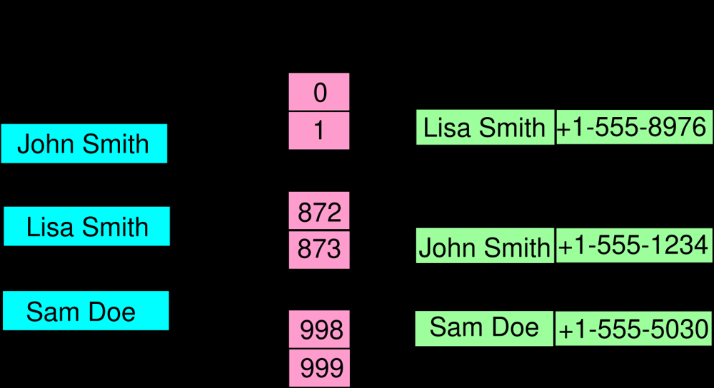
A hash table is a data structure that provides very fast average-case lookup of keys by using a hash function to compute an index. Searching in a hash table involves computing a hash code from the key and then checking the corresponding bucket or slot for the item.

How it works: A hash table maintains an array of “buckets.” When inserting a key (often associated with a value), the key is run through a hash function – an algorithm that deterministically converts the key into a numerical index (usually an integer). This index corresponds to a position in the underlying array. The item is stored in that position. To search for a key, the same hash function is applied to the key, yielding an index; you then look at that index in the array to find the key’s value.

Because different keys can produce the same hash index (a collision), hash tables implement collision resolution strategies:

In separate chaining, each array index holds a linked list (or another structure) of entries that hashed to that index. Upon collision, the new entry is appended to the list in that bucket. Searching involves hashing to the bucket, then traversing a small list of candidates to find an exact match.
In open addressing, if an index is occupied, the algorithm probes to find another free slot (using schemes like linear probing, quadratic probing, or double hashing). Searching then follows the same probe sequence until either the key is found or an empty slot is encountered (meaning the key is not in the table).

Hash Table example. This diagram illustrates a hash table storing phone numbers for people by name. The names (“John Smith”, “Lisa Smith”, “Sam Doe”) are run through a hash function to determine indices (shown in pink). Each index points to a slot that holds the actual key-value entry (name and phone number, shown in green). In this example, two names hashed to the same index range, demonstrating a collision that the hash table must handle (in a real hash table, this could be resolved by chaining or probing). Despite collisions, lookups are efficient because we only search within a small localized area of the table.

Time complexity: The power of hash tables is in their average-case performance. A well-implemented hash table offers O(1) average time complexity for search, insertion, and deletion – constant time on average, independent of the number of elements. This assumes a good hash function that distributes keys evenly and that the load factor (ratio of number of entries to number of buckets) is kept in check (often by resizing the table when it becomes too full). In the worst case, however, hash table search can degrade to O(n) time – for instance, if all keys collide into the same bucket, a search might have to scan through all entries in a list.

Use cases: Hash tables are ubiquitous in software development whenever a fast lookup by key is needed:

Dictionaries/Maps: Most programming languages provide a dictionary (or map) data type implemented with a hash table (e.g., Python’s dict, Java’s HashMap, C++’s unordered_map). This allows quick search of values by keys like strings, identifiers, etc.
Databases and Caches: In memory caching systems or database indexing (when keys are not sorted), hash tables allow rapid retrieval of records by key. For example, a cache of web page contents might use URLs as keys hashed to quickly find the cached page data.
Symbol tables/Compiler: Compilers use hash tables to manage identifiers (variables, function names) so they can quickly check if a name has been declared or lookup its attributes.
Sets: A set data structure (which just tracks presence/absence of elements) is often implemented as a hash table on the element key, providing O(1) membership tests.

Hash tables are favored for their average performance and simplicity of use. One must choose a good hash function for the key type to minimize collisions and be mindful of resizing strategies to maintain efficiency. With proper implementation, searching in a hash table is extremely fast and often close to constant time for practical sizes.

Trie Search

A Trie (pronounced “try”, also known as a prefix tree) is a tree-like data structure that is particularly useful for searching strings or sequences by their prefixes. Each node in a trie represents a prefix of some keys, and edges typically correspond to individual characters (or components) of keys.

How it works: In a trie, the root node represents an empty string. Each edge out of the root represents the first character of some keys. As you go down levels, you accumulate characters. Each node may have multiple children, one for each possible next character in keys that share the prefix up to that node. For example, consider a trie storing the words “cat”, “cap”, and “dog”:

The root has branches for ‘c’ and ‘d’.
Under ‘c’, there is a node for the prefix “ca”, which then branches into ‘t’ and ‘p’ for “cat” and “cap”.
Under ‘d’, there’s a node for “do”, branching to ‘g’ for “dog”.

To search for a key (e.g., the word “cap”) in a trie, you start at the root and follow the sequence of child pointers corresponding to each character of the key:

Start at root (prefix = “”).
For each character in the search string, go to the child node labeled with that character.
If at some point, the required child does not exist, the search fails (the key is not in the trie).
If you consume all characters and reach a node that marks the end of a stored key, the search is successful.

Because each step in the search goes to the next character’s node, the time to search is proportional to the length of the key (not the number of keys in the trie).

Trie example. — Trie example: The image above shows a trie containing the words “to”, “tea”, “ted”, “ten”, “A”, “i”, “in”, and “inn”. Each node (circle) represents a prefix. For instance, the path spelling “ten” leads to a node marked as a complete word (with an associated value, shown in blue). Searching for a word involves tracing down from the root through successive letters. For example, to find “ten”, we start at the root, follow ‘t’ to node “t”, then ‘e’ to node “te”, then ‘n’ to node “ten”, which is marked as a word. If a path exists for all characters and the final node indicates a valid key, the search is successful. Tries naturally handle prefix queries too; for example, finding all words that start with “te” would involve locating the node for “te” and exploring its subtree (“tea”, “ted”, “ten” in this case).

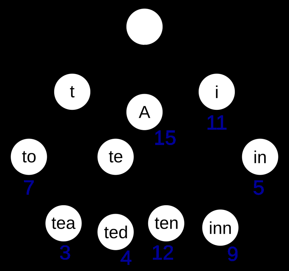
Time complexity: Searching for a key of length m in a trie is O(m) in the worst case. This is independent of how many keys are stored, as it only depends on the length of the key being searched. This makes tries very efficient for search operations, especially when keys are long and share prefixes. In the example above, searching “inn” would take 3 steps (for ‘i’ -> ‘n’ -> ‘n’), regardless of whether the trie stores 10 words or 10 million words, as long as those steps exist. The flip side is space: tries can consume a lot of memory, since they potentially have a node for every prefix of every key, and sparse branches for uncommon prefixes can lead to many null or empty children pointers.

Use cases: Tries are ideal for applications that involve prefix-based searches or need to store a large vocabulary of strings:

Autocomplete and Spell-checking: When you start typing in a search bar, the system can traverse a trie of dictionary words according to your input and suggest completions by exploring that node’s descendants. Tries enable retrieving all words with a given prefix efficiently.
Dictionary and word games: Word-based puzzles, like crosswords or Boggle solvers, use tries to quickly test prefixes and words. It’s easy to check if a prefix is valid (leads to some word) or if a word exists by traversing the trie.
IP routing and network packet forwarding: Tries (in the form of Patricia tries or radix trees) are used to store routing prefixes (like IP address prefixes) so that longest prefix matching can be done quickly to decide where to route a packet.
DNA sequence storage: In bioinformatics, tries can store DNA sequences (composed of A, C, G, T characters) to allow quick lookup of patterns or prefixes within a database of sequences.

While tries excel in speed for searches and prefix operations, they do have overhead in terms of memory. Various optimizations like compressed tries (or radix trees) collapse single-child sequences to save space, and bitwise tries handle binary data efficiently. Nonetheless, the direct character trie is conceptually straightforward and powerful for search tasks where keys have a sequential structure (like strings).

Binary Search Tree Search

A Binary Search Tree (BST) is a binary tree data structure that keeps elements in sorted order, allowing search, insertion, and deletion operations in average logarithmic time. Each node in a BST has up to two children, often referred to as left and right, and it satisfies the BST property: all nodes in the left subtree of a node have values less than that node’s value, and all nodes in the right subtree have values greater.

How it works: The BST property guides the search algorithm:

Start at the root node of the tree.
If the target value equals the value at the current node, the search is successful.
If the target value is less than the current node’s value, move to the left child and continue the search there (because by BST property, the left subtree contains smaller values).
If the target value is greater than the current node’s value, move to the right child (the right subtree has larger values).
Continue this process down the tree. If you reach a leaf (null child pointer) without finding the target, the value is not present in the tree.

This procedure is essentially a binary search performed on the tree structure instead of an array. Each comparison allows the algorithm to discard half of the remaining tree (all nodes on one side).

For example, consider a BST containing the numbers 8, 3, 10, 1, 6, 14, 4, 7, 13 (inserted in that order). The BST might be structured with 8 at the root, 3 as left child of 8, 10 as right child of 8, and so forth (3’s left child 1, 3’s right child 6, etc.). If we search for the value 7:

Start at root (8). 7 < 8, so go left.
At node 3. 7 > 3, so go right.
At node 6. 7 > 6, so go right.
At node 7. We found 7, success.

Time complexity: The time complexity for search (and insert/delete) in a BST is O(h), where h is the height of the tree. In a balanced BST, the height h is O(log n) for n nodes, so searches take O(log n) on average. However, in the worst case, if the tree becomes skewed (like a linked list – which can happen if we insert already sorted data into an unbalanced BST), the height becomes O(n) and search time degrades to O(n).

Balanced binary search trees (like AVL trees, Red-Black trees, B-Trees, etc.) have extra rules or rotations to keep the height minimal, ensuring consistently good performance. Many library implementations of sets and maps are backed by balanced BSTs (e.g., C++ std::map typically uses a Red-Black tree).

Use cases: BSTs are useful when you need to maintain a dynamically changing set of comparable items and be able to search, insert, and delete efficiently:

In-memory databases or indices: If you need data sorted and also need fast lookups, a BST can maintain sorted order and allow binary-search-like performance for lookups. For example, a BST could index user records by username for quick search by username, while also allowing iteration of all usernames in sorted order.
Implementing sets/maps: Many language libraries use self-balancing BSTs for ordered collections. Anytime you use a sorted associative container (like a TreeMap in Java or a sorted set), under the hood, a BST is performing the search operations.
Symbol tables in compilers (alternative): While hash tables are often used, BSTs (especially balanced ones) can be used for symbol tables to get ordered traversal of symbols (if needed) in addition to fast search.
Networking and OS: BSTs can be used in implementing certain caches or lookups where ordering is important (though specialized trees or tries often handle IP routing or interval searches more directly).

One important advantage of BSTs over hash tables is that BSTs maintain elements in sorted order, so you can perform range queries (find all entries between X and Y) efficiently by traversing the tree – something not directly possible with hash tables. Balanced BSTs guarantee that the performance remains good even in the worst case, making them reliable for applications requiring consistent responsiveness.