Physical Address
304 North Cardinal St.
Dorchester Center, MA 02124
Physical Address
304 North Cardinal St.
Dorchester Center, MA 02124

This comprehensive guide demystifies search algorithms, from simple linear scans to hash‑table lookups, tries, balanced trees, and BFS/DFS in graphs. All while showing you how each strategy slashes lookup time for specific data shapes and teaching you how to write efficient code.
Searching algorithms are fundamental in computer science for finding a specific item or piece of information within a larger collection of data. The efficiency of a search algorithm often hinges on its time complexity – how the number of operations grows with the size of the data. A linear time approach (denoted O(n)) will check elements one by one, so the work grows in direct proportion to the number of items. In contrast, a logarithmic time approach (O(log n)) dramatically reduces comparisons by halving the search space at each step. For example, locating a name in an unsorted list might require scanning each entry (linear search), whereas finding it in a sorted directory can be done in far fewer steps by repeatedly narrowing the range (binary search). Choosing between linear vs logarithmic search methods depends on whether the data is organized in a way that allows skipping large portions during the search.
Modern software employs a variety of searching algorithms optimized for different scenarios. Some algorithms work on simple arrays or lists, some leverage specialized data structures for faster lookups, and others are designed to traverse complex structures like graphs. Below, we organize the algorithms into categories and explain each in detail, including how they work, their mechanics, and real-world use cases.
Choosing the right searching algorithm depends on the data structure and the specific problem at hand. For simple collections, basic algorithms like linear or binary search might suffice, with binary search being preferred for sorted data due to its logarithmic efficiency. Specialized structures like hash tables, tries, and binary search trees offer tailored search performance — constant time lookups in hash tables, prefix-based retrieval in tries, and ordered searches in trees — at the cost of additional memory or maintenance overhead. In scenarios where data forms complex networks, graph search algorithms like DFS and BFS become indispensable for traversing or finding specific nodes, with BFS providing shortest paths in unweighted scenarios and DFS enabling deep exploration.
In practice, understanding these algorithms and the patterns of access they optimize for allows developers to make informed decisions: whether it’s worth sorting data to enable binary search, using a hash table for instant key-based access, or building a trie for auto-completion features. The goal is always to reduce search time and handle data efficiently. By leveraging the appropriate search strategy, programs can achieve significant performance gains, especially as data size scales into large volumes. Each algorithm in this collection is a tool – knowing when and how to use it is a fundamental skill in software engineering and computer science.
This article is part of a comprehensive guide about algorithms. To access the main article and read about other types of algorithms, from sorting to machine learning, follow the following link:
A Friendly Guide to Computer Science Algorithms by Category.
These algorithms operate on linear collections (such as arrays or lists). They range from the straightforward linear scan to more complex methods that exploit sorted order to achieve faster lookups.
Linear search (also known as sequential search) is the simplest method to find a target value in a list. The algorithm starts at the first element and checks each item one by one until the target is found or the list ends. If the item is found, the search can terminate early; if not, the algorithm concludes after examining every element.
How it works: Imagine searching for a book by title on an unsorted shelf. A linear search would have you examine each book in order until you find the one you want. In pseudocode form, it’s essentially:
for each element in list:
    if element == target:
        return FOUND
If the target equals the current element, the search stops successfully; otherwise it moves to the next element.
Time complexity: Linear search runs in O(n) time in the worst and average cases (where n is the number of elements). This means the search time grows linearly with the data size. For example, searching 1000 items might in the worst case require 1000 comparisons. Linear search does not require any special data ordering or preprocessing.
Use cases: Linear search is practical for small or unsorted datasets. When the collection is tiny or performance requirements are low, the overhead of more complex algorithms isn’t justified. It’s also the fallback method for data structures like linked lists (which do not support efficient random access) – you must traverse node by node to find a value. In everyday programming, you might use linear search to check if a value exists in an array that isn’t sorted. Another common scenario is scanning an array or file for a particular value (e.g., finding a specific word in a short list of strings). While linear search is simple, its inefficiency becomes apparent as data sizes grow, which motivates algorithms with better-than-linear performance.
Binary search is a much faster algorithm for finding an element in a sorted array or list. By leveraging the sorted order, binary search eliminates half of the remaining elements in each step, achieving a logarithmic time complexity.
How it works: Binary search operates by repeatedly dividing the search interval in half:
For example, suppose you have a sorted list of names and you want to find “Smith”. Binary search would compare “Smith” to the middle name in the list. If “Smith” comes alphabetically after that middle name, you can ignore the entire first half of the list and focus on the second half; if “Smith” comes before the middle, you discard the second half and focus on the first half. In a list of 1000 sorted names, a binary search would require at most about 10 comparisons (since 2^10 ≈ 1024) to either find the name or conclude it’s not present – a stark contrast to up to 1000 comparisons in linear search.
Time complexity: Binary search runs in O(log n) time. Each comparison cuts the remaining search space in half, so the number of steps grows logarithmically with the number of elements. However, binary search requires that the data be sorted beforehand (or maintained in sorted order). There is a space trade-off as well: binary search can be implemented iteratively with O(1) extra space or recursively with O(log n) stack space.
Use cases: Binary search is widely used for any lookup operation on sorted data. Real-world applications include:
binary_search in C++ STL, Arrays.binarySearch in Java) for efficient searching in sorted arrays – these all use binary search internally.Jump search is an algorithm designed for searching in sorted arrays by checking fewer elements than linear search, making “jumps” through the array. The idea is to skip ahead by fixed steps and perform a linear search within a smaller block, rather than checking every element in sequence.
How it works: Given a sorted array of length n, you choose a fixed jump size m. Typically, an optimal jump size is the square root of the array length (m ≈ √n), which balances the number of jumps and the linear checks within a block. The algorithm proceeds as follosw:
For example, suppose you have a sorted list of 10,000 numbers and you set a jump size of 100. You would check elements at indices 0, 100, 200, 300, … until the value at an index exceeds the target. If the target is, say, within index 200 to 299, the jump search will find that the element at 300 is larger than the target, so it knows the target must be between 200 and 299. It then linearly scans that smaller range to find the exact index of the target.
Time complexity: In the optimal case where the jump size is √n, jump search will perform about √n jumps and at most √n linear steps in the final block, yielding a time complexity of roughly O(√n). This is better than O(n) of linear search but worse than O(log n) of binary search. In fact, jump search’s complexity falls between linear and binary search. The advantage of jump search is that it minimizes backward movement. It mostly moves forward through the array and only does a short linear scan at the end.
Use cases: Jump search is less commonly used in practice than binary search, but it can be advantageous in scenarios where jumping ahead sequentially is efficient and random access is not too costly, yet we want to avoid multiple random jumps backward. One real-world scenario could be searching on disk storage or tape where sequential reads are fast but random seeks are expensive – jump search will perform mostly sequential reads. For instance, if data is stored on a medium like a magnetic tape or a sequential-access file, you might “jump” forward in chunks to narrow down where a record is, then read sequentially around that area instead of doing binary search which would involve jumping back and forth. Overall, while binary search is usually preferred for in-memory array searches, jump search provides a conceptual alternative that highlights the trade-off between skipping through data and scanning short sections linearly.
Interpolation search is an improvement over binary search for sorted arrays of numbers when the values are uniformly distributed (or roughly so). Instead of always checking the middle of the remaining range as binary search does, interpolation search attempts to estimate the position of the target based on the target’s value relative to the range of values.
How it works: The algorithm computes an estimated position using a linear interpolation formula. Given a sorted array arr[low...high] and a target value x, the position is estimated as:
pos = low + ((x - arr[low]) * (high - low) / (arr[high] - arr[low]));
This formula guesses where the target might be within the current range by assuming the values increase roughly linearly. Essentially, if x is closer to arr[low], it will choose a position near the beginning of the range; if x is closer to arr[high], it will pick a position near the end. After computing pos, the algorithm compares arr[pos] to the target:
arr[pos] is the target, it returns the index.arr[pos] is smaller than the target, it means the target should lie to the right of pos (so set low = pos + 1 and continue).arr[pos] is larger than the target, it means the target is to the left of pos (so set high = pos - 1 and continue).Because interpolation search uses the data distribution, it will zoom in faster on the target position when values are uniformly distributed. For instance, if you have a telephone directory and you want to find the entry for “Smith”, binary search would start at the middle, but interpolation search might jump closer to the “S” section immediately by calculating the likely position of “Smith” relative to “AAA…” and “ZZZ…”.
Time complexity: The average-case complexity of interpolation search is O(log log n) when values are uniformly distributed. This is better than binary search’s O(log n) in those ideal conditions. However, the worst-case complexity is O(n) (for example, if the data distribution is highly skewed or if every element is the same except the target). In the worst case, the interpolation formula might always choose poor split points (like always picking one end of the range), degrading to a linear scan.
Use cases: Interpolation search is useful in situations where comparisons are cheap and the data is known to be fairly uniform. A classic example is searching for a record by key in a uniformly distributed numerical database (like finding a record by an evenly distributed ID number). It’s more of a theoretical interest algorithm; most real systems still prefer binary search because it guarantees O(log n) worst-case. However, for something like looking up a word in a alphabetically evenly distributed list or searching in a file where entries are uniformly distributed in key space, interpolation search can outperform binary search. In practice, its use is limited because data rarely has a perfectly uniform distribution, but it’s an important concept that demonstrates how exploiting value distribution can speed up search.
Exponential search (also known as doubling search or search in an infinite array) is an algorithm that works on sorted arrays and is particularly useful when the size of the array is unknown or unbounded. It combines the idea of increasing range exploration with binary search.
How it works: Exponential search has two stages:
x and you found that arr[k] is the first element >= x (or you ran off the end of the array at index k). Then you know the target, if present, lies between index k/2 and k.[k/2, k] is identified (inclusive of boundaries), perform a binary search on that sub-array to locate the target precisely.As an example, imagine an infinite sorted list of numbers (or one that you don’t know the length of). You want to find if a number x exists in it. Exponential search would first check index 1, 2, 4, 8, 16, … doubling each time, until it either finds the number or finds a number larger than x (or hits an out-of-bound if length is finite but unknown). Say it finds that at index 16 the number is 50 and is >= x (and at index 8 the number was 30 which was < x). Now it knows x lies between index 8 and 16. Then it does a binary search in that interval to find x.
Time complexity: Exponential search runs in O(log n) time. The range-finding phase takes O(log n) steps because you double the index each time (the index grows exponentially until exceeding n or the target’s position). Once the range is found, binary search inside that range takes another O(log n) in the worst case. Overall, that’s O(log n + log n) = O(log n). In practice, the doubling phase adds a constant factor 2 overhead to the binary search phase. The advantage is that you don’t need to know the array size beforehand, and if the target is near the beginning of the array, exponential search finds it very quickly (even faster than a full binary search would, because the range found might be very small).
Use cases: Exponential search is particularly useful when dealing with unbounded or infinite-length arrays (or data streams). A typical scenario is an infinite sorted stream of data where you want to find a certain value without reading everything. Another use is in libraries or systems where you can’t easily get the size of the list but can probe it (for example, searching through a very large file that you memory-mapped, or in a scenario like binary search on a sorted, but streaming, dataset). Some database or search engine implementations might use exponential search as a strategy to find bounds for binary search on disk-based sorted data. It is also used in algorithms that require searching within a bounded but unknown size structure – for example, in competitive programming problems where the array size isn’t given but you know it’s sorted, you can use exponential search to avoid having to guess the size.
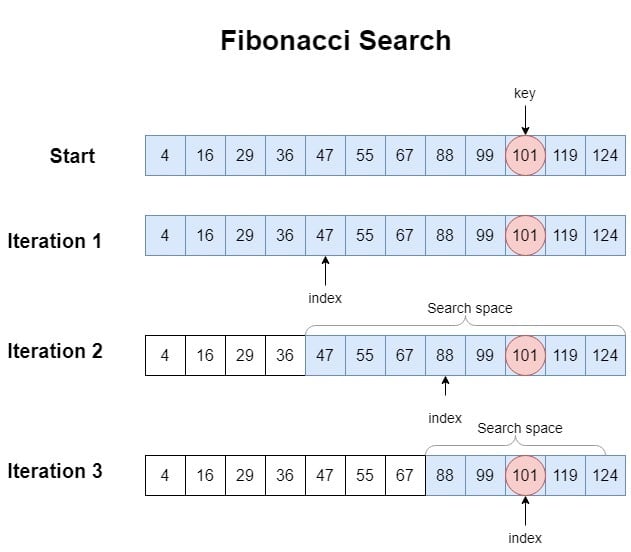
Fibonacci search is another divide-and-conquer search algorithm for sorted arrays, similar to binary search but using Fibonacci numbers to split the range. It’s a comparison-based technique that sometimes can have performance benefits on certain systems due to the pattern of index access (though in Big-O terms it is equivalent to binary search).
How it works: Fibonacci search maintains a range size that is a Fibonacci number. It determines the fibonaccis F(k) that bounds the array length (n). For example, find the smallest Fibonacci number that is >= n. The idea is to use Fibonacci numbers to partition the array:
F(k) be the smallest Fibonacci number >= n. Set offset = -1 (this marks the start of the range being considered; initially none of the array is eliminated).offset + F(k-2) (which is a roughly 2/3 position, since F(k-2) is two Fibonacci numbers down from F(k)) with the target.
offset + F(k-2), and reduce k by 1 (because we eliminate the lower portion).F(k-1), then F(k-2), etc.) to probe positions, until the range size becomes 1 or the target is found.In essence, Fibonacci search uses predetermined positions based on the Fibonacci sequence to check elements, rather than always the middle. The sequence gives a systematic way to divide the array.
Time complexity: Fibonacci search runs in O(log n) time, similar to binary search. The number of comparisons will be around log₁.₆₁₈(n) (where 1.618 is the golden ratio, since Fibonacci numbers grow exponentially at rate φ≈1.618), which is of the same order as log₂(n). So in pure complexity terms, there’s no big difference from binary search. However, Fibonacci search may have slightly different comparison patterns which in some cases could align better with memory access patterns.
Use cases: Historically, Fibonacci search was discussed in contexts where certain computational models made it perform better than binary search by a constant factor. For example, on systems where arithmetic operations were costly but simple addition/subtraction was cheaper, Fibonacci search avoids division by 2 (which binary search does to find mid) and uses only addition/subtraction. In modern times, those differences are negligible, and binary search is usually preferred for simplicity. Fibonacci search is mostly of academic interest, showing an alternate way to do binary-like searching. It might be used in cases where the cost of computing midpoints is non-trivial or when trying to avoid division operations, but such scenarios are rare with today’s hardware. Understanding Fibonacci search can deepen insight into how we can use different mathematical strategies (like Fibonacci numbers) to guide search intervals.
The algorithms above consider searching in plain arrays or lists. However, data is often stored in more complex structures that offer their own search mechanisms. These structures are designed to improve search efficiency by storing information in ways that facilitate quick lookups.
Access the Search Algorithms for Data Structures following this link.
In contrast to searching within linear structures or hierarchical trees, graph search algorithms deal with traversing a general graph (which could be thought of as a network of connected nodes). Two fundamental graph search strategies are Breadth-First Search (BFS) and Depth-First Search (DFS). These algorithms systematically explore nodes and edges of a graph to find a target or to traverse all reachable nodes from a starting point. While they are often used for “traversal” (visiting all nodes) rather than direct key-based lookup, they are essential whenever the data forms a graph or network.
Access the Graph-Based Search Algorithms following this link.
To go to the main guide about algorithms follow this link: A Friendly Guide to Computer Science Algorithms by Category,